Basic Practice

I. Knowledge Framework

In this chapter we will use the basic Python libraries pandas, numpy and matplotlib to complete a small data analysis project. It is recommended to practice with jupter-notebook in the Anaconda environment.

II. Background

This is a set of airline customer data, and we hope to extract valuable information from it. The data is as follows.

chapter2-1.zip

III. Analysis Method

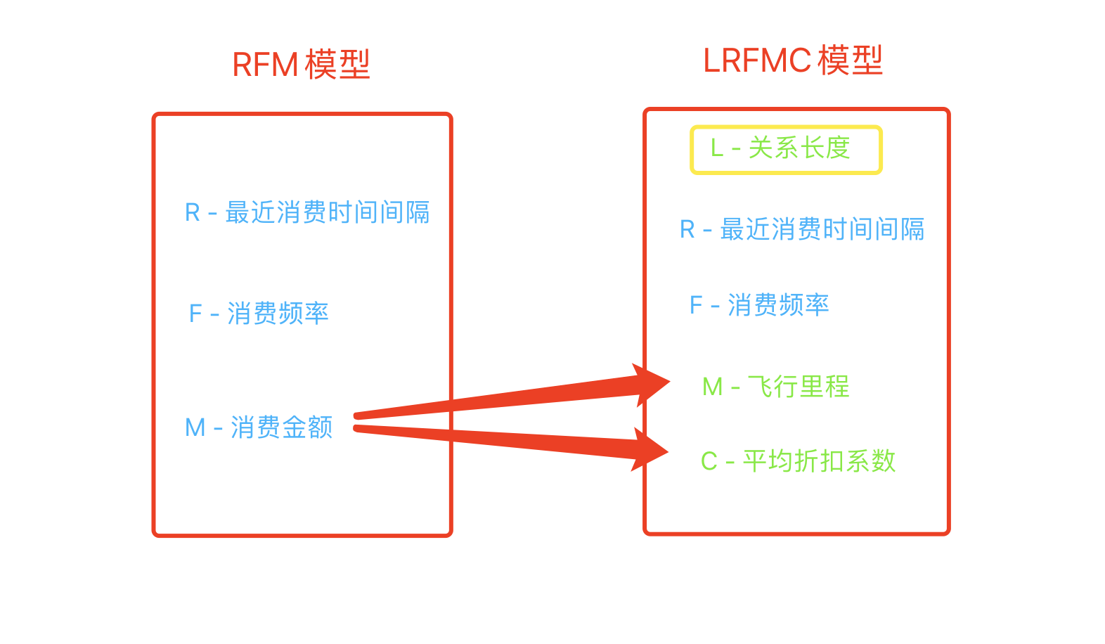
For customer analysis, a widely used method is the RFM model, where R stands for recency (the interval since the most recent purchase), F stands for frequency (purchase frequency), and M stands for money (amount spent). Considering our project, if one customer bought a discounted long-haul ticket and another bought a short-haul ticket in a premium cabin, their spending may be the same, but the customer who bought the premium cabin ticket is clearly more valuable. So we replace the amount spent with M-mileage (flight mileage) and C-coefficient (discount coefficient), and add a parameter L-long (relationship length), which represents the time since joining the membership program. In this way, we modify the RFM model into the LRFMC model.

IV. Analysis Process

Let’s review the analysis process, which mainly consists of the following five steps:

Data source - obtained from the business system
Data extraction - extract historical data
Data exploration - explore missing values and outliers in the data
Data preprocessing - clean and transform the data
Data modeling - build a machine learning model
Result feedback - provide strategies

Next, what we need to do is data exploration

V. Exploratory Analysis

We can easily find the missing values, maximum values and minimum values in the data with the following code

import pandas as pd

# 1 Define the file names
datafile = 'air_data.csv'  # Original file
resultfile = 'explore.csv'  # Target file

# 2 Read the file data
data = pd.read_csv(datafile, encoding='utf-8')  # Use pd.read_csv to read the csv file

# 3 Present the file content
explore = data.describe().T  # Get the descriptive statistics and then transpose the matrix

# 4 Count the number of blanks
explore['null'] = len(data) - explore['count']

# 5 Build the problem matrix
explore = explore[['null', 'max', 'min']]  # Use this matrix to get a first look at the problems

# 6 Rename the matrix columns
explore.columns = ['空值数量', '最大值', '最小值']

# 7 Save the exploration file
explore.to_csv(resultfile)

VI. Data Preprocessing

Data preprocessing mainly uses data cleaning and data transformation, which are prerequisites for building the model. The principles of data cleaning must be determined by the business scenario. Based on the business scenario, we set the following rules: keep records where the ticket price is non-zero, or where the average discount rate is non-zero and the total flight mileage is greater than zero, and then clean the data. The code is as follows

import numpy as np
import pandas as pd

# 1 Read the raw data
datafile = 'air_data.csv'
cleanedfile = 'data_cleaned.csv'
data = pd.read_csv(datafile)
print("原始数据的形状", data.shape)

# 2 Drop missing data
airline_notnull = data.loc[data['SUM_YR_1'].notnull() & data['SUM_YR_1'].notnull()]
print("删除缺失数据后的形状", airline_notnull.shape)

"""
3 定制规则：保留票价非零数据，或平局折扣率不为零且总飞行里程大于零的数据，然后清洗数据
"""
index1 = airline_notnull['SUM_YR_1'] != 0  # Keep non-zero ticket prices
index2 = airline_notnull['SUM_YR_2'] != 0
index3 = airline_notnull['SEG_KM_SUM'] > 0  # Keep flight mileage greater than zero
index4 = airline_notnull['avg_discount'] != 0  # Keep non-zero average discount rates

# Keep ages under 100
index5 = airline_notnull['AGE'] < 100

# Combine the conditions
airline = airline_notnull[(index1 | index2) & index3 & index4 & index5]
print("清洗后的数据形状", airline.shape)

# Save the data
airline.to_csv(cleanedfile)

VII. Data Transformation

Data standardization is the last step of preprocessing: the data format needs to be transformed into what the model requires.

I must keep working hard to get there, so that I can meet you as the best version of myself, and I hope you will be the same.

# L Relationship length - LOAD_TIME - FFP_DATE
# R Recency (interval since the most recent purchase) - LAST_TO_END
# F Purchase frequency - FLIGHT_COUNT
# M Flight mileage - SEG_KM_SUM
# C Average discount coefficient - AVG_DISCOUNT

# Data standardization
import pandas as pd
import numpy as np

cleanedfile = 'data_cleaned.csv'
data = pd.read_csv(cleanedfile)

# Select the required attributes
airline_selection = data[['LOAD_TIME', 'FFP_DATE', 'LAST_TO_END', 'FLIGHT_COUNT', 'SEG_KM_SUM', 'avg_discount']]

# Look at the first five rows
airline_selection.head()

# Compute the value of L
L = pd.to_datetime(airline_selection['LOAD_TIME']) - pd.to_datetime(airline_selection['FFP_DATE'])
L.head()

# Convert the data type of L
L = L.astype('str').str.split().str[0]
L.head()
L = L.astype('int') / 30
L.head()

# Merge the computed L with the attributes above that need no computation
airline_features = pd.concat([L, airline_selection.iloc[:, 2:]], axis=1)
airline_features.head()

# Rename the columns
airline_features.columns = ['L','R','F','M','C']
airline_features.head()

# Standardization: can be understood as (original value - mean) / standard deviation
from sklearn.preprocessing import StandardScaler
data = StandardScaler().fit_transform(airline_features)

np.savez('airline_scale.npz', data)

data[:, :5]

VIII. Data Modeling

Once standardization is complete, the next step is data modeling. Building the customer value analysis model consists of two main parts. First, cluster customers into groups based on the five indicators, that is, gather similar people together; the benefit is that later we can apply the same marketing strategy specifically to each group. Second, analyze the characteristics of each customer group in light of the business, rank the customer groups, and analyze customer value, so that subsequent strategies give priority to serving the top-ranked important customers.

We use the kmeans algorithm to perform the cluster analysis. The analysis process is as follows

from sklearn.cluster import KMeans
import matplotlib.pyplot as plt

airline_scale = np.load('airline_scale.npz')['arr_0']

k = 5  # Set k to the number of groups you want to divide similar objects into

# Build the model
kmeans_model = KMeans(n_clusters = k, random_state=123)  # random_state is the random seed

# Train the model
fit_means = kmeans_model.fit(airline_scale)

# Get the cluster centers
kmeans_cc = kmeans_model.cluster_centers_
print(kmeans_cc)  # Each row represents a point in five-dimensional space

# Get the sample cluster labels
kmeans_labels = kmeans_model.labels_
print(kmeans_labels)

# Count the number of samples in each cluster
r1 = pd.Series(kmeans_labels).value_counts()

# Convert the data format
cluster_center = pd.DataFrame(kmeans_model.cluster_centers_, columns=['L','R','F','M','C'])

# Reset the order
cluster_center.index = pd.DataFrame(kmeans_model.labels_).drop_duplicates().iloc[:,0]
print(cluster_center)  # Use the clustering algorithm to group tens of thousands of users into 5 clusters

As for the clustering algorithm, we don’t need to worry about how it works for now; we will have a dedicated chapter on it later. For now, just follow my code and understand the process step by step.

IX. Data Visualization

Pure numbers make it hard for us to observe the results of the cluster analysis, so let’s use data visualization to draw them as a chart and take a look.

import matplotlib.pyplot as plt

labels = ['L','R','F','M','C']  # Indicators
legen = ['customer' + str(i + 1) for i in cluster_center.index]  # Names
lstype = ['-','--',(0,(3,5,1,5,1,5)),':','-.']  # Styles

kinds = list(cluster_center.iloc[:,0])  # Categories
kinds

# Close the data loop; a radar chart needs closed data
cluster_center = pd.concat([cluster_center, cluster_center[['L']]], axis=1)
cluster_center

centers = np.array(cluster_center.iloc[:, 0:])
centers

# Length for dividing the circle
n = len(labels)

angle = np.linspace(0,2*np.pi, n, endpoint=False)
angle = np.concatenate((angle, [angle[0]]))
angle

# Canvas
fig = plt.figure(figsize=(8,6))
ax = fig.add_subplot(111, polar=True)

for i in range(len(kinds)):
    ax.plot(angle, centers[i], linestyle=lstype[i], linewidth=2, label=kinds[i])

    ax.set_thetagrids(angle*180/np.pi, labels)
plt.title('customer type')

plt.legend(legen)  # Add the legend
plt.show()

X. Writing an Analysis Report Based on the Business

The moment to show the skills of an excellent data analyst has arrived. All the work we did above was for this final step: analyzing customer value, follow-up strategies and marketing plans in the context of the business scenario is the most important part of data analysis.

L Relationship length - LOAD_TIME - FFP_DATE
R Recency (interval since the most recent purchase) - LAST_TO_END
F Purchase frequency - FLIGHT_COUNT
M Flight mileage - SEG_KM_SUM
C Average discount coefficient - AVG_DISCOUNT

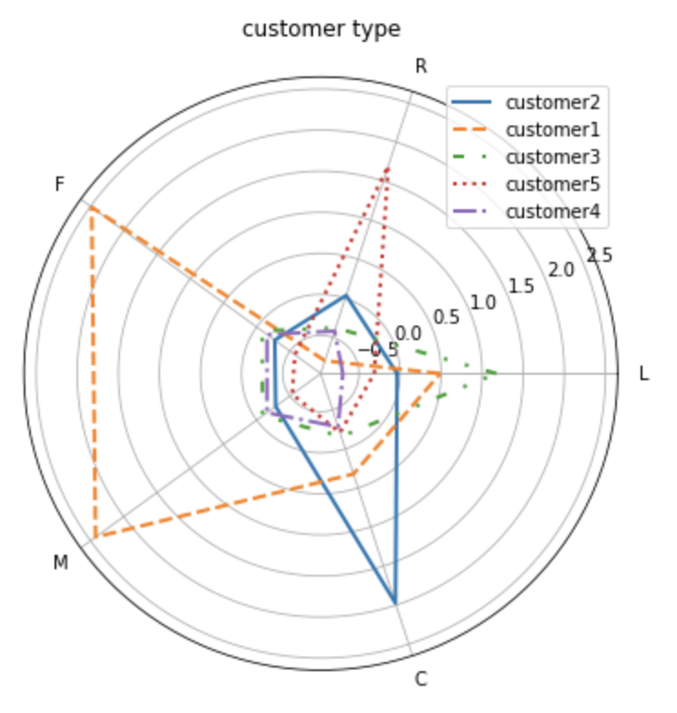
We’ve put the chart and the indicator for each dimension here; now let’s analyze based on the chart together. The feature analysis chart above shows that each type of customer has distinctly different characteristics. Based on the description of these characteristics, we divide these customers into five levels of customer categories: important customers to retain, important customers to develop, important customers to win back, and general customers. The characteristics of each customer category are as follows:

Important customers to retain: customer1. These customers have a high average discount rate (C), indicating that they generally fly in higher cabin classes; their time since last flying with this airline (R) is low, and their number of flights (F) and mileage (M) are the highest. They are the airline’s high-value customers, the most ideal customer type, and contribute the most to the airline, yet they account for a small proportion. The airline should prioritize putting resources into them, apply differentiated management and one-to-one service, improve their loyalty and satisfaction, and extend their high level of spending as long as possible.
Important customers to develop: customer2. These customers have the highest average discount rate. Although their current value is not high, they are potentially valuable customers for the airline. The airline should work to get them to spend more, strengthen customer satisfaction, raise their cost of switching to competitors, and gradually turn them into loyal customers of the company.
Important customers to win back: customer3. These customers have been members the longest, but their other attributes are relatively low. The airline should adopt certain marketing measures based on changes in these customers’ most recent purchase time and number of purchases, to extend the customer lifecycle.
General-value customers: customer4, customer5. These customers have no loyalty to speak of; they probably only buy when tickets are discounted.

XI. Supplementary Analysis

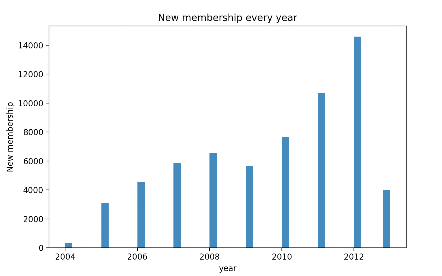
1 Number of New Members Each Year

import pandas as pd
from datetime import datetime
import matplotlib.pyplot as plt

data = pd.read_csv('air_data.csv')
ffp = data['FFP_DATE'].apply(lambda x: datetime.strptime(x, '%Y/%m/%d'))
ffp_year = ffp.map(lambda x: x.year)
fig = plt.figure(figsize=(8, 5))
plt.rcParams['font.sans-serif'] = 'SimHei'
plt.rcParams['axes.unicode_minus'] = False
plt.hist(ffp_year, bins='auto')

plt.xlabel('year')
plt.ylabel('New membership')
plt.title('New membership every year')
plt.show()

The result is shown in the figure below:

2 Male-to-Female Ratio Analysis

male = pd.value_counts(data['GENDER'])['男']
female = pd.value_counts(data['GENDER'])['女']

fig = plt.figure(figsize=(7, 4))
plt.pie([male, female], labels=['male', 'female'])
plt.title('male and female')
plt.show()

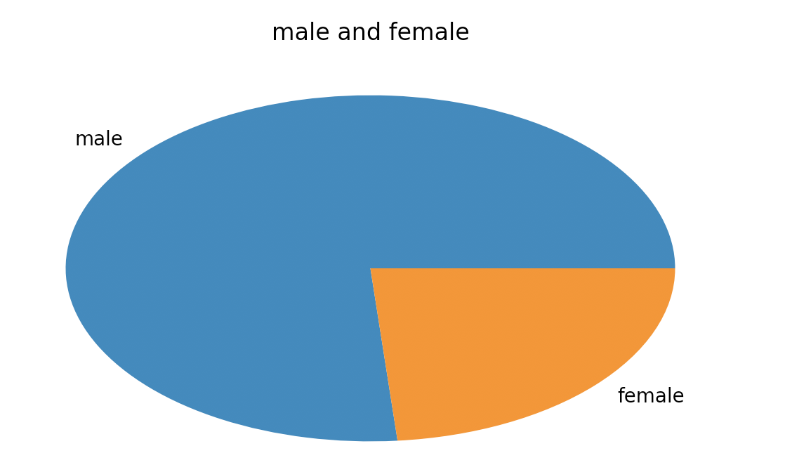
The result is shown in the figure below:

These are some of the most commonly used charts. Of course, there are many more charts waiting for us to learn later. For every kind of data there is always a chart suited to representing it, so data visualization plays a very important role in data analysis and the AI field. I believe that through this chapter, you will be able to master the entire data analysis process and gain a whole new understanding of data.